temperature_response

hinode.xrt.temperature_response(filter, time, abundance='coronal', variance=False, axis_filter='filter', axis_temperature='temperature')

The temperature response of XRT through the given filters on a given date, as xrtpy computes it.

This is the response of xrtpy.response.TemperatureResponseFundamental: the CHIANTI spectrum distributed with xrtpy folded with the effective area of each filter [Narukage et al., 2011], including the contamination of the CCD and of the filters on that date.

Parameters:

• filter (str | Sequence[str] | AbstractScalarArray) – The filters to return the response of, named as in hinode.xrt.urls(), such as "Al_poly" or "Al_poly/Ti_poly". If a string or a sequence of them, the filters are put along axis_filter.

• time (str | Time) – The date of the observation, which sets the thickness of the contamination.

• abundance (str) – The abundances of the CHIANTI spectrum, "coronal", "hybrid", or "photospheric".

• variance (bool) – If True, the response is the variance of the signal due to the counting of the photons, rather than the signal, so that the ratio of the two responses is the factor which sets the photon noise of hinode.xrt.Filtergram.uncertainty().

• axis_filter (str) – The name of the axis along the filters, if filter does not already have one.

• axis_temperature (str) – The name of the axis along the temperatures of the result.

Returns:

• A function of temperature whose outputs are the response of each filter

• to unit emission measure, in

• \(\text{DN}\,\text{cm}^5\,\text{s}^{-1}\,\text{pix}^{-1}\),

• or in \(\text{DN}^2\,\text{cm}^5\,\text{s}^{-1}\,\text{pix}^{-1}\,\text{ph}^{-1}\)

• if variance is True.

Return type:

FunctionArray[ScalarArray, ScalarArray]

Notes

The coronal spectrum distributed with xrtpy 0.5 was computed with CHIANTI 10.0, and the hybrid and photospheric spectra with CHIANTI 9.01, as the metadata of their files say, all at a constant electron density of \(10^9\,\text{cm}^{-3}\) and at log temperatures from 5 to 8 in steps of 0.05. The temperature response of the AIA channels in sdo uses another version of CHIANTI at a constant pressure, so a DEM found from both instruments is usually allowed a factor between the two responses.

Each photon of wavelength \(\lambda\) gives a signal \(s = h c / (\lambda w G)\), where \(w\) is the energy needed to free an electron and \(G\) is the gain of the CCD. The response is the sum over wavelength of the rate \(n\) at which the CCD absorbs photons times their signal, \(R = \sum n s\), which is the sum xrtpy.response.TemperatureResponseFundamental.integration() takes. The number of photons is a Poisson variable and their signals differ, so the variance of the signal grows at the rate \(R_\sigma = \sum n s^2\), and the variance of a pixel is its signal times \(R_\sigma / R = \langle s^2 \rangle / \langle s \rangle\), which is larger than the average signal of one photon, \(\langle s \rangle\).

Examples

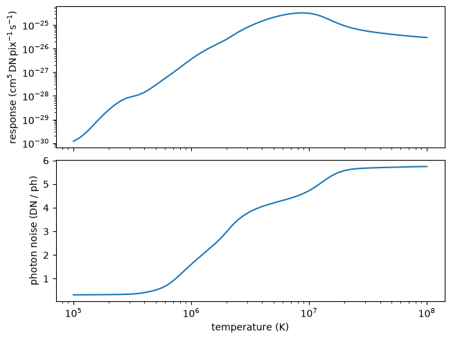
The response of the Al_poly filter on the date of the flight of the EUV Snapshot Imaging Spectrograph (ESIS), and the factor which sets the photon noise at each temperature.

import matplotlib.pyplot as plt
import astropy.units as u
import astropy.visualization
import named_arrays as na
import hinode

response = hinode.xrt.temperature_response("Al_poly", "2019-09-30")
variance = hinode.xrt.temperature_response(
    filter="Al_poly",
    time="2019-09-30",
    variance=True,
)

index = dict(filter=0)

with astropy.visualization.quantity_support():
    fig, axs = plt.subplots(
        nrows=2,
        sharex=True,
        constrained_layout=True,
    )
    na.plt.plot(
        response.inputs,
        response.outputs[index],
        ax=axs[0],
        axis="temperature",
    )
    na.plt.plot(
        response.inputs,
        (variance.outputs / response.outputs)[index],
        ax=axs[1],
        axis="temperature",
    )
    axs[0].set_xscale("log")
    axs[0].set_yscale("log")
    axs[0].set_ylabel(f"response ({response.outputs.unit:latex_inline})")
    axs[1].set_ylabel("photon noise (DN / ph)")
    axs[1].set_xlabel(f"temperature ({response.inputs.unit:latex_inline})")